
|
Geological Survey Professional Paper 1044—C
The Waters of Hot Springs National Park, Arkansas—Their Nature and Origin |
THE HOT-SPRINGS FLOW SYSTEM
The geologic, hydrologic, and water-chemistry data and interpretations presented in previous sections of the report provide the bases from which a conceptual model of the hot-springs flow system can be formed. Digital models of the flow system provide a test of the conceptual model and a vehicle for further refinement of the conceptual model.
CONCEPTUAL MODEL
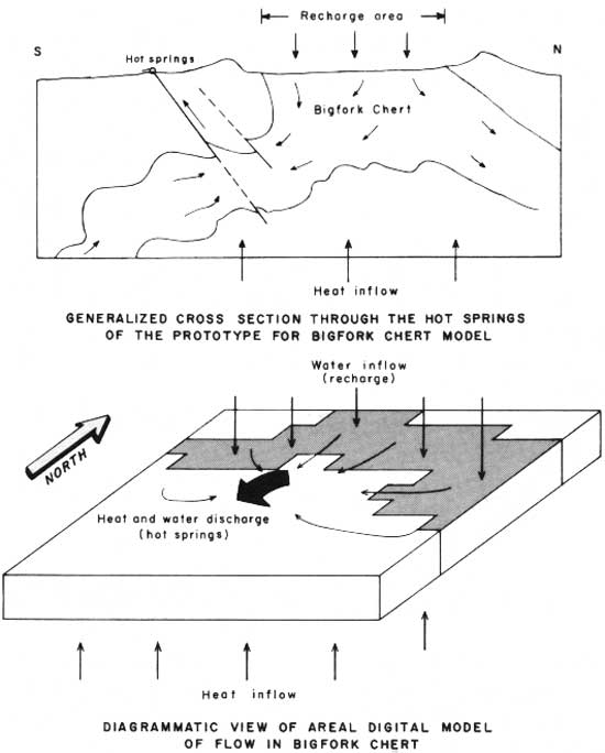
The hot-springs water is meteoric; that is, it is derived from precipitation. The water is recharged to formations in the hot-springs region (within a few tens of miles), as opposed to being recharged to formations distant (several tens or hundreds of miles) from the hot springs. The origin and proximity of recharge of the hot-springs water are revealed by the chemical constituents and isotopes in the water and the flow variations of the hot springs.
The formation or formations that form the recharge area must possess the following general characteristics:
1. The outcrop area must be relatively large and permeable, that is, from 3 to 10 mi2 (7.77 to 25.9 km2), assuming permeabilities that would permit average recharge rates of from 2 to 6 in (50.8 to 152.4 mm) per year.
2. The elevations of water levels in the recharge area must be high enough to provide hydraulic head for spring flow. The springs emerge at elevations ranging from 576 to 683 ft (175.6 to 208.2 m) above mean sea level.
3. The recharge formations must be hydraulically connected to the permeable zones that feed the springs.
Consideration of the lithology and structure of rocks in the area reveals two formations whose outcrops may serve as recharge areas—the Bigfork Chert and the Arkansas Novaculite. The outcrop area of the Bigfork Chert meets several of the requirements of the hot-springs recharge area—the Bigfork crops out over an area of about 36 mi2 (93.2 km2) north and northeast of the hot springs, in the area shown in figure 6. The Bigfork Chert generally possesses moderately high fracture and intergranular permeability. Faults and fracture zones are common. Permeable zones extending from the Bigfork Chert to the hot springs could be provided by faults (pl. 1) that connect the Bigfork Chert with permeable zones in the Arkansas Novaculite and the Hot Springs Sandstone Member of the Stanley Shale or that provide a permeable fault zone through the Missouri Mountain and the Polk Creek Shales to the hot springs.
The Arkansas Novaculite crops out in the vicinity of the hot springs in a smaller area than does the Bigfork Chert (fig. 6). Within the mapped area in figure 6, the outcrop of the Arkansas Novaculite covers about 13 mi2 (33.7 km2). Permeability of the Arkansas Novaculite varies greatly; in places it is moderately high. The outcrop of Arkansas Novaculite occupies the highest elevation in the vicinity of the hot springs.
The elevation of head in the recharge area required to provide hot-spring flow depends on such factors as transmissivity of the aquifer, areal extent of the recharge area, distance of the recharge area from the springs, depth of flow of water en route to the springs, and the temperature of the water in the aquifer. These factors, except for the effect of temperature on hydraulic head, are accounted for in the digital models of the aquifer. The effect of the increased temperature of water in the flow system reduces the head required in the recharge area to drive the system. The density of water above 4.0°C (39.2°F) decreases as its temperature increases. Water at 61.7°C (143.1°F) (average hot-springs temperature) is 98 percent as heavy as water at 17.7°C (63.9°F) (average temperature of recharge water). Therefore, a column of water at 17.7°C (63.9°F), 1,000 ft (304.8 m) in length, will support a 1,020-ft (310.8 m) column of water at 61.7°C (143.1°F). It would be possible for a thermal artesian system to have a lower water-level elevation in the recharge area than in the discharge area. However, under conditions of uniform areal heat flow, it would not be possible for artesian flow to be initiated without sufficient head in the recharge area to drive the system.
Water levels in the outcrop area of the Bigfork Chert range from a few feet above land surface (flowing wells) to 30 ft (9.14 m) below land surface. Water levels in the Arkansas Novaculite range from a few feet above land surface to 50 ft (15.2 m) below land surface. As an approximation of the area in which heads in the Big fork Chert and the Arkansas Novaculite are at a minimum to sustain flow in the artesian system, the outcrop area above 700 ft (213.4 m) mean sea level was chosen. Within the area shown in figure 6, about 8.5 mi2 (22.0 x 10⁶ m2) of the outcrop of Bigfork Chert is above 700 ft (213.4 m) mean sea level, and almost all the outcrop of Arkansas Novaculite is above 700 ft (213.4 m) mean sea level. However, under about 5 mi2 (13.0 x 10⁶ m2) of the Arkansas Novaculite outcrop, the northwest limit of the anticline north of the hot springs, the formation dips northwestward and probably is not in a favorable structural position to supply water to the hot springs.
Analysis of streamflow provides information on the magnitude of recharge. Stream discharge and rainfall records have been collected on three small basins in the vicinity of the hot springs (Bedinger and others, 1974). The locations of the gages on East Fork and West Fork of Hot Springs Creek are shown in figure 6. The gage on Glazypeau Creek is located about 9 mi (14.5 km) north-northeast of the hot springs. Each basin is relatively small and is underlain principally by Bigfork Chert. The Arkansas Novaculite underlies the higher elevations of East Fork and West Fork of Hot Springs Creek (fig. 6).
Base flow is ground-water discharge to the stream and is derived from recharge of precipitation. A relatively large part of rainfall on the Bigfork Chert outcrop recharges the subsurface reservoir. Base flows in the East and West Forks of Hot Springs Creek are 61 and 84 percent, respectively, of precipitation (Bedinger and others, 1974). These figures are primarily a measure of the recharge to the Bigfork Chert. Also, the base-flow studies indicate that interbasin transfers of ground water occur. Such interbasin transfers of ground water, probably from several stream basins, supply the water to the hot springs.
The large surface area, the great capacity to admit recharge, and the relatively high permeability of the Bigfork suggest that the Bigfork Chert is the principal recharge source to the hot-springs artesian system. The Arkansas Novaculite has a smaller outcrop area of potential recharge, a lower capacity to admit recharge, and a generally lower permeability. However, the Arkansas Novaculite is probably a source of part of the recharge to the hot-springs system. Further analysis of the Bigfork Chert and Arkansas Novaculite as the recharge sources and principal aquifers of the flow system is made in the section on modeling.
The 14C age of the hot-springs water averages 4,430 years. The greater part of the time that the water is in underground circulation the movement is very slow. That is, movement is on the order of a few feet to a few tens of feet per year and is distributed through a large volume of the aquifer. This slow movement of water continues to relatively great depths in the aquifer and probably includes lateral circulation where sufficient heat is absorbed to reach temperatures greater than 60°C. This heat is supplied by conduction through adjacent rocks of lower permeability. In the absence of fluid circulation, heat is conducted toward the land surface at rates near 1.2 x 10⁻⁶ calories per second per centimeter squared, or 1.2 heat-flow units in most of the Eastern United States. In areas of abnormally high crustal radioactivity, the geothermal heat flow may be as high as 2.2 heat-flow units (M. L. Sorey, written comm., 1976). On the basis of an assumed thermal conductivity of 0.006 calorie per second per centimeter squared and heat flow of 1.2-2.0 heat-flow units, the normal geothermal temperature gradient in the vicinity of the hot springs should be between 0.006°C/ft and 0.01°C/ft, although the available subsurface temperature information is insufficient to confirm these gradients. With these gradients and a maximum spring temperature at depth of 63°C based on silica concentrations, the minimum depth of fluid circulation would range from 4,500 to 7,500 ft.
Highly permeable zones, probably related to jointing or thrust faulting, collect the heated water in the aquifer and provide avenues for the water to travel to the surface. Rapid movement of the water from depth to the surface is indicated by the very small decrease in temperature from the maximum temperature attained at depth to the temperature at the surface.
DIGITAL FLOW MODELS
The purpose of modeling the hot-springs flow system was to test several hypotheses regarding the nature of the flow system. Each hypothesis requires details of aquifer geometry and various combinations of hydrologic variables, such as area and depth of circulation, hydraulic conductivity, and porosity. The model analysis provides a means for estimating values of these variables that can be compared with observed data for the hot springs (such as temperature, discharge, 14C concentration, and silica concentration).
The equation for the heat-flow model is
| H = KN ( | XD |
((X1 - X0)( | MA1+MA0 |
)+(X3-X0) |
| YD | 2 |
| ( | MA3+MA0 |
)) + | YD |
((X2-X0 )( | MA2+MA0 | )+ |
| 2 | XD | 2 |
| (X4-X0)( | MA4+MA0 |
)) + (XD)(YD) |
| 2 |
| ( | TTOP - X0 + DH0 |
)) |
| DP0 |
+ SP ( X1Q1+X2Q2+X3Q3+X4Q4-X0QO)
The subscripts in the preceding equation refer to node location (a node is the center of a volume element); 0 refers to the nodal location being considered, 1 refers to the node above, 2 refers to the node to the right, 3 refers to the node below, and 4 refers to the node to the left. In the preceding equation, H is the heat-flow residual, in British thermal units per day; KN is the thermal conductivity, in British thermal units per day-foot-degree Fahrenheit; X is the temperature, in degrees Fahrenheit; XD is the horizontal node spacing, in feet; YD is the vertical node spacing, in feet; MA is the thickness of the aquifer (equivalent to thickness of the model), in feet; TTOP is the temperature at land surface, in degrees Fahrenheit; DP is the depth to the midpoint of the aquifer (average of the depth to the top and the depth to the base), in feet; DH is the temperature gradient at the base of the aquifer, in degrees Fahrenheit per foot; SP is the volumetric specific heat of water, 62.4 British thermal units per degrees Fahrenheit-cubic foot (4.18 x 10⁶ joules per degrees Celsius-cubic meter); Q1, 2, 3, 4 is the inflow of water from node 1, 2, 3, and 4, respectively, in cubic feet per day; and Q0 is the outflow of water from the element, in cubic feet per day.
The equation for the ground-water-flow model is
| QT = | XD |
(( | P1MA1+P0MA0 |
)(S1-S0)+ |
| YD | 2 |
| ( | P2MA2+P0MA0 |
)(S3-S0)) |
| 2 |
| + | YD | (( | P2MA2+P0MA0 |
)(S2-S0)+ |
| XD | 2 |
| ( | P4MA4+P0MA0 |
)(S4-S0)) |
| 2 |
QT is the ground-water flow residual, in cubic feet per day; P is the hydraulic conductivity, in feet per day; and S is the ground-water potential (head), in feet. Other symbols and the subscripts are as explained for the heat-flow model.
DESCRIPTION OF THE HYDROTHERMAL MODEL
The heat-flow and ground-water flow models are based on the equations of continuity for heat and water, respectively. That is, the net flux of heat, or water, into an element of volume is equal to the change in heat, or water, concentration of the element. Under steady-state conditions, neither temperature nor head change with time, and the net flux of heat, or water, into any element of the model is equal to zero. The equation of continuity for heat, or water, is written for each of the elements of the model. If there are N elements in the model, the result is N linear equations in N unknown temperatures, or heads. These N linear equations are solved by (1) assuming an initial temperature, or head; (2) using the Jacobi iteration method to calculate new values for temperature, or head; and (3) calculating the residual for each element. The residual is the sum of the head, or water, inflow to each element. The residual would be zero for each element if the N temperatures, or heads, were exact solutions of the N equations. The initial values used were 18.3°C (64.9°F) for the heat-flow model and 0 ft head for the ground-water flow model. Steps 2 and 3 are repeated until the sum of all the residuals in the model is less than 0.1 percent of the total flux in the model. The total flux is equal to the total heat inflow to the heat-flow model, or to the total recharge for the ground-water flow model.
According to R. O. Fournier (oral commun., 1972), the relation between saturated silica concentration and temperature is
| MGL = 60,060 (10 -( | 1,032 | + 0.09)), |
| K |
where MGL is the silica concentration at saturation with chalcedony, in milligrams per liter; and K is the temperature, in degrees Kelvin (°C+273.2). The assumptions made in the model of silica concentration are: (1) If the water is supersaturated with silica (silica concentration greater than that given by the preceding equation), the silica will remain in solution and not precipitate; (2) if the water is undersaturated with silica (silica concentration less than that indicated by the preceding equation), sufficient silica will go into solution so that the water becomes saturated with silica. The effect of these two assumptions requires that the water either be saturated or supersaturated with silica. The iterative procedure for calculating the silica distribution in the aquifer is as follows. First, the silica concentration at a node was calculated from the inflow by
| SIL = | Q1S1L1+Q2SIL2+Q3SIL3+Q4SIL4 |
, |
| Q1+Q2+Q3+Q4 |
where SIL is the silica concentration at a node as calculated from the inflow, in milligrams per liter; SIL1 2,3, 4 are silica concentrations at surrounding nodes, in milligrams per liter; and Q1, 2, 3, 4 are inflows (zero, if outflow) from surrounding nodes, in cubic feet per day. Subscripts are as defined in the heat-flow equation. The silica concentration at the node is chosen as the larger of SIL, given previously, or MGL, as given in the previous equation. On the first iteration, all the silica values are as given by the equation for MGL. Succeeding iterations produce silica values as weighted from inflow by the equation for SIL. An indicator is kept for the maximum change in silica from one iteration to the next. When this indicator becomes less than 0.0001, the final silica values have been computed and the iteration is stopped.
The iterative procedure for calculating time of travel uses the equation
| TT = | Q1TT1+Q2TT2+Q3TT3+Q4TT4+ |
| ||
| Q1+Q2+Q3+Q4 + (B) (XD) (YD) | ||||
(D1(MA1+MA0)+D2(MA2+MA0)+D3(MA3+MA0)+D4(MA4+MA0) ),
where TT is the time of travel, in years; D is one if the corresponding Q is positive and zero if the corresponding Q is zero; POR is the porosity, dimensionless; and B is the recharge rate at the node, in feet per day. Other symbols and the subscripts are as defined previously. An indicator is used that is the maximum change in time of travel from one iteration to the next. When this indicator becomes less than or equal to 0.0001, the iteration is stopped.
The model for 14C is based upon the exponential decay of 14C, a radioactive isotope of carbon. This decay can be expressed as
C14t=C14 e -(1.2097 X 10⁻⁴) t
where C14 is the initial 14C content, C14t is the 14C concentration after a period of time has elapsed, and t is the elapsed time, in years. The recharge area of the aquifer is not the only source for the carbon in the water, as some carbon is added by solution of aquifer material. As table 9 shows, within the bulk of the system, only 55 to 65 percent of the carbonate present is 14C bearing. The 14C model uses 65 percent as an initial value and decreases this value according to the exponential decay. The 14C model is an iterative procedure calculating 14C from the equations
Q1C14teA1+Q2C142eA2+Q3C143eA3
| C14 = | +Q4C144eA4+B (XD) (YD) |
| Q1+Q2+Q3+Q4+B (XD) (YD) |
and
(-1.2097 x 10⁻⁴) (XD) (YD) (POR)
| Ai = | (MA1+MA0), i = 1,2,3,4 , |
| 730 Qi |
where C14 is the 14C concentration, in percent of modern as measured, and other symbols and subscript meanings are as used previously. An indicator is used whose value is the maximum change of C14 from one iteration to the next. When this indicator becomes less or equal to 0.0001, the iteration is terminated.
APPLICATION OF DIGITAL MODELS TO THE HOT-SPRINGS FLOW SYSTEM
Most of the data on the hot-springs flow system, such as water temperature, water samples for analysis, and flow measurements, have been collected from points at or near the Earth's surface. Subsurface data are from wells, the deepest of which is about 336 ft (102.4 m). Conditions at depth must be inferred by such means as projection of surface dips of rock formations and faults and changes in temperature and chemical nature of the water from the recharge area to the springs. The digital models provide a further tool with which conditions at depth can be inferred. Measured properties of the flow system and the water can be entered into the digital model. The flow model provides simultaneous solutions to the equations for each of the several properties. The design of the system at depth can be changed experimentally within the bounds of known parameters so that the model results are compatible with all measured properties related to the system.
Following is a summary of variables that must be specified in designing a steady-state model of the flow system.
1. Thickness, porosity, hydraulic conductivity, and depth of the aquifer.
2. Thermal conductivity of the rocks and heat flow into the aquifer.
3. Recharge to the aquifer.
4. Temperature of water in the recharge area.
The initial flow models were designed from projections of surface dips of the geologic formations and from known and estimated hydrologic and thermal properties of the aquifer. Two flow models were designed and tested during the study. In one model the Bigfork Chert served as the principal aquifer. In the other model the Arkansas Novaculite served as the principal aquifer. During development of each model, the design was changed in attempting to achieve harmony between the input data and the known constraints on the system.
The Bigfork Chert was modeled as a two-dimensional plane, inclined in the subsurface to the southeast (fig. 12). The flow of water was modeled to a point in the subsurface beneath the spring discharge area. Flow upward to the surface was not modeled because the model is limited to a two-dimensional representation of the flow system. Temperature and silica data on the hot springs indicate that the flow of water from depth to the surface is relatively rapid. That the flow from depth to the surface was not modeled is not considered significant with regard to conclusions drawn from the model. Following is a summary of the input data for the Bigfork Chert model.
| Thickness of aquifer | ft. | 1,500 |
| Porosity | 0.20 | |
| Hydraulic conductivity at 18.3°C (nonuniform) | ft/d | 0.5-10 |
| Thermal conductivity | cal/s-cm°C | 0.006 |
| Heat flow (nonuniform) | hfu | 2.2-22.0 |
| Recharge rate (nonuniform) | ft/yr | 0.05-0.25 |
|
| FIGURE 12.—Model of flow in the Bigfork Chert. |
The Bigfork Chert in the model is thicker than the average reconstructed stratigraphic thickness for this formation. However, the Bigfork Chert contains multiple folding, which increases the actual thickness of the water-bearing zone. Also, the underlying Womble Shale contains permeable zones of limestone and chert which effectively increase the thickness of the contiguous water-bearing zone. The hydraulic conductivity of the Bigfork Chert was modeled as 1 ft/day (3.53 x 1026 m/s) over the outcrop area and in most of the subsurface. The higher values of hydraulic conductivity were modeled in a zone trending east-northeast from the hot springs, parallel to the trace of the thrust faults through the hot-springs area (fig. 2). The hydraulic conductivity in the model, after being adjusted by the program to reflect the temperature of the water, ranged from 1 to 25 ft/day (3.53 x 1026 to 8.82 x 1025 m/s). The maximum depth of water circulation in the model is 6,000 ft (1,830 m). Heat was added at the lower surface of the model at rates of 2.2 hfu over most of the model area and 22.0 hfu over the area near the springs. Heat was removed from the upper surface of the model at rates calculated from the product of thermal conductivity and the temperature difference between each node and the assumed land-surface temperature of 18.3°C divided by the depth of the node. The abnormally high heat flows of 22.0 hfu near the springs and 2.2 away from the springs were necessary to achieve the observed temperature at the springs. Results of the model are summarized in table 10.
TABLE 10.—Comparison of the modeled and observed data for the hot springs using the Bigfork Chert as the principal aquifer
| Parameter | Modeled | Observed | |
| Temperature | °C | 61.2 | 61.7 |
| Flow | ft3/d | 0.97 X 10⁵ | 1.1 X 10⁵ |
| Silica | mg/L | 40.7 | 41.7 |
| Carbon-14 age | yr | 5,026 | 4,430 |
| Maximum head in recharge area above hot springs | ft | 18 | 260 |
The results of the Bigfork Chert model indicate that the known and assumed values of the parameters are within the hydrologic constraints on the system. The model indicates that the available head difference is ample to provide the hydraulic pressure for the spring flow. An additional component of head is produced by the decreased density of the water at temperatures higher than the assumed temperature in the recharge area (18.3°C (64.9°F) ). The ample head available to drive the flow system provides a leeway in several of the estimated values of parameters used in the model, such as thickness and permeability of the aquifer and rate and areal extent of the recharge. For example, a valid model could be designed using lower values for permeability and thickness of the Bigfork Chert, or a valid model could be designed using a lower recharge rate over a larger area or using a higher recharge rate over a smaller area.
The critical constraint on the Bigfork Chert model is the high heat flow needed to obtain the observed spring temperature. It was not possible to obtain the 62°C—discharge temperature using a uniform heat inflow of 2.2 hfu, which as discussed previously is the maximum known value of crustal heat flow in the Eastern United States. This heat-inflow deficiency suggests consideration of an alternative model of the Bigfork Chert in which the ground-water flow system supplying the hot springs absorbs heat throughout a larger area.
The Arkansas Novaculite was modeled as a nearly vertical two-dimensional plane inclined slightly to the southeast (fig. 13). Flow was modeled to a point in the subsurface near the springs from which flow to the surface is probably rapid and through a very permeable zone. Following is a summary of input data for a model of the Arkansas Novaculite:
| Thickness of aquifer | ft | 500 |
| Porosity | 0.1 | |
| Hydraulic conductivity | ft/d | 1. |
| Thermal conductivity | cal/s-cm-°C. | 0.0062 |
| Heat flow | hfu | 2.2 |
| Recharge rate | ft/yr. | 0.63 |

|
| FIGURE 13.—Model of flow in the Arkansas Novaculite. |
Results of the Arkansas Novaculite model are summarized in table 11. One constraint on this model is that the required difference in head between the recharge area and the springs (1,222 ft, or 372 m) exceeds the available head by a factor of 3. This required head difference is also much larger than the head provided by the water level in the recharge area (420-ft, or 128-m, maximum) and the temperature differential (estimated to be about 160 ft, or 49 m).1 Known values of hydraulic conductivity of the Arkansas Novaculite indicate that the average value cannot reasonably be expected to exceed 1 ft/d, 0.30 m/d, (at 18.3°C) throughout an area as large as that modeled.
1For=0.02 and L=8,000 ft, δH=0.02 (8,000 ft)= 160 ft, where δp is the change in density, p0 is the initial density of the water, L is the depth of circulation, and δH is the heed provided by the temperature differential.
TABLE 11.—Comparison of the modeled and observed data for the hot springs using the Arkansas Novaculite as the principal aquifer
| Parameter | Modeled | Observed | |
| Temperature | °C | 54.4 | 61.7 |
| Flow | ft3/d | 0.85X10⁵ | 1.1X10⁵ |
| Silica | mg/L. | 36.0 | 41.7 |
| Carbon-14 age | yr | 2,760 | 4,430 |
| Maximum head in recharge area above hot springs | ft | 1,222 | 420 |
The Arkansas Novaculite model could also be rejected on structural considerations. To obtain a discharge temperature within 10 percent of the observed spring temperature, the depth of circulation in the novaculite model was 8,000 ft (2,440 m), and heat was added over the lower surface of the slightly inclined plane, 1.52 by 26 mi, or 40 mi2 (2.45 by 41.8km, or 102.4 km2) (as indicated in fig. 13) at a uniform rate of 2.2 hfu and removed over the upper surface of the plane at rates proportional to the temperature difference between each node and the land surface. Structurally, a continuous aquifer in the Arkansas Novaculite with this lateral extent and depth is of doubtful validity.
DISCUSSION OF MODELS
Neither the Bigfork Chert model nor the Arkansas Novaculite model, previously described, is entirely satisfactory in describing the hot-springs flow systems. In terms of hydrologic and structural constraints on the model, the Arkansas Novaculite model is the least plausible, whereas the Bigfork Chert model is the most suitable. In terms of thermal considerations, both models require abnormally high heat flow to achieve the observed temperature of the hot springs.
An alternative Bigfork Chert model, which could match the observed discharge temperatures with observed heat flows in the Eastern United States, would involve lateral circulation of ground water over an area on the order of 50 mi2, which, in turn, would require that the recharge areas be distributed over a larger region than in the Bigfork Chert described previously. Recharge from distances as great as 5-10 mi would probably be sufficient. Such a flow system may be possible along the plane of the thrust fault(s) that intersects the hot springs and dips to the northwest (pl. 1). The criteria for the recharge areas along the thrust fault(s) would be that recharge occur at distances as great as 5-10 mi north and northeast of the hot springs at elevations above the spring discharge and that there be hydraulic connection with the fault plane at sufficient depth to allow water to move laterally toward the springs. Ground water movement would be relatively slow to the point where it intercepts the thrust fault plane. Movement along the fault plane would be relatively rapid to the points of spring emergence. Such a model would meet the age requirements indicated by 14C analyses.
| <<< Previous | <<< Contents >>> | Next >>> |
pp/1044-C/sec3.htm
Last Updated: 09-Mar-2009